Okay, let’s get a little closer to understanding what the derivative really is.

Rate of Change for a Series of Time Intervals

What I propose we do next is plot the battery charge rate of change for a range of time intervals over our day’s battery state of charge curve. We will generate a list of start points and calculate the rate of change for some interval from each start point.

For now I am going to start by refactoring rate_chg(c_fn, t1, t2) to include an additional paramter, dt. This will specify the value to add to t1 to get the end of the range for the rate of change. I.E. get the rate of change for \(t1\) to \(t1 + dt\).

I will be calculating the series of time values for which to determine the rate of change in the function. Hence, \(t2\) is still needed. The range of times will be from \(t1\) to \(t2\) at some specified interval. As in previous code, we will be using np.arange to generate the series of times. \(dt\) will also be used to specify the distance between the points in the series. E.G. \(1.0\) hour.

... ...
# code control vars
do_soc = False
do_roc = False
do_s_roc = True
... ...
def roc_series(c_fn, t1, t2, dt):
  '''
  Determine rate of change for a series of two times on the curve generated by c_fn.
  
  :param c_fn: function to use to produce values for the two points
      for which the rate of change is wanted
  :param t1: start time
  :param t2: end time for series
  :param dt: amount time separating times in generated series of times
             also used to generate end time for calculating rate of change
             for each time in the series

  Returns: times in the generated series, est rate of change for each time
  '''
  ts = np.arange(t1, t2, dt)
  roc = [rate_chg(c_fn, t, t+dt)[0] for t in ts]
  return ts, roc
... ...
if do_s_roc:
  # generate and plot rate of change for a series of times
  t_btwn = 1
  ts, roc = roc_series(soc_fn, 0, 24, t_btwn)
  for i, tm in enumerate(ts):
    print(f"{tm}: {roc[i]}")

And in the terminal…

(mc-3.14) PS R:\learn\mc\calculus> python p_p1.py
0.0: -9.3
1.0: -8.7
2.0: -7.5
3.0: -5.7
4.0: -3.6
5.0: -1.2
6.0: 1.2
7.0: 3.6
8.0: 5.7
9.0: 7.5
10.0: 8.7
11.0: 9.3
12.0: 9.3
13.0: 8.7
14.0: 7.5
15.0: 5.7
16.0: 3.6
17.0: 1.2
18.0: -1.2
19.0: -3.6
20.0: -5.7
21.0: -7.5
22.0: -8.7
23.0: -9.3

Okay, let’s plot that so we can actually see what is going on.

... ...
import math
... ...
  # quick plot
  yl = (math.floor(min(roc)), math.ceil(max(roc)))
  xl = (0, 24)
  ax.set(xlim = xl, 
         ylim = yl,
        autoscale_on = False)
  ax.scatter(ts, roc)
  ax.set(xlabel='Time of Day (hr)', ylabel='Change Rate (% / hr)',
        title='Estimated Battery Charge Rate for a Series of Times')
  ax.grid()

  plt.show()

And, the result…

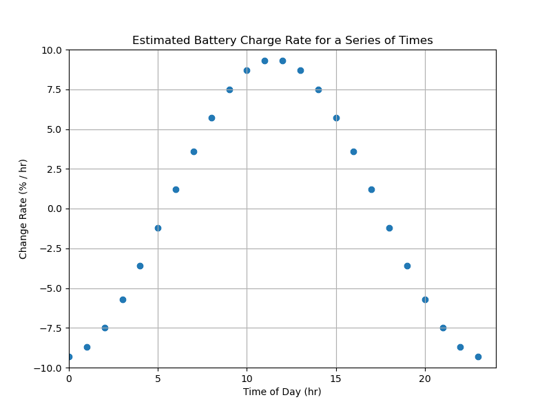
And, that seems to make sense. In the original state of charge plot, the state was increasing from approximately 06:00 to 18:00. And, decreasing everywhere else during the day. Albeit at different rates for any given point in time. And a peak increasing rate of change around noon, makes a certain amount of sense. Especially if no one is home at the time. Assuming people were home, I would expect that peak to be a couple of hours later.

Plot the Actual Differential

Time to add the curve of the actual differentiated function to the plot.

No I am not going to show you the code for that. No calculus—remember? You’ll just have to take my word the curve added to the plot is generated by the equation for the differential of our state of charge function. Function, df_soc(t), coded to provide the value of the differential for any given time(s).

If you are really interested see Calculus II: Appendix.

Here’s the relevant code.

... ...
if do_s_roc:
  do_real_df = True
... ...
  # added alpha value so that line plot does disappear in the scatter plot
  ax.scatter(ts, roc, alpha=.3)
... ...
  if do_real_df:
    # dc_dhr = (-3 * np.pi) * np.cos(np.pi * hr / 12)
    t = np.arange(0.0, 24.0, 0.05)
    dc_dh = df_soc(t)
    ax.plot(t, dc_dh, c="k")
    d_font = {'color':  'black',
        'weight': 'bold',
        'size': 12
        }
    plt.text(16, 5.5, f"plot of differential", fontdict=d_font)
    # fig.savefig("bat_roc_3.png")

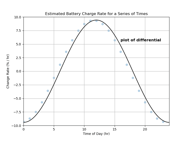
Not a bad match given we are calculating the rate of change between two points 1 hour apart. And the differential gives us the instantaneous rate of change at any point in time.

Tighten the Time Interval for the Rate of Change Plot

Let’s see what happens when we reduce that hour spacing we were using to generate the scatter plot. Which, effectively, is an estimate of the plot of the differential. Let’s say every 15 minutes, t_btwn = 0.25 # 15 minute intervals.

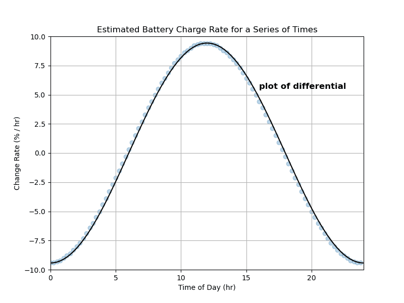
Well, still not a perfect match; but, certainly very much closer. Do you perhaps see where we are heading?

Time to Take a Break

A short post and I have not yet completed this journey of discovering the differential. That should leave another relatively short post for next time.

Until then, enjoy your time playing with arithmetic and graphical plots.