As mentioned in a previous post, I had intended to code a function to generate the rate of change curve for a day. Normally, would just use the equation for the state of charge derivative over some range of times to generate the plot. But, we are trying to do this without any actual calculus. So, let’s have a look at that, before we move on with our look at calculus.

We did in fact sort of do this in the last post,, using a loop. But let’s refine things a little with a suitable function or two. Yes, juz cuz. Though there is perhaps an ulterior motive.

Function for Rate of Change

We want something that is going to give us the rate of change for a range of times. Which we will then plot.

The function to generate the data for the curve is going to need a number of parameters—at least during development. May be able to get rid of some of them after things are working as desired. I.E. by hardcoding the best values in the function.

As running our differential estimation function can take some time depending on the degree of precision desired, I am going to have a paramater to control that value. I am also going to need parameters for the function—estimating the rate of change a some point in time—and the start and end times. Additionally, I am thinking, at least during development, to include a parameter for the total number of data points between the two times. That will also affect how long the function takes to generate the desired data for the plot.

Now we have the function est_df(fn, hr, n_dec=6) but it only works for a single time. So our new function will repeatedly call this function in order to generate the number of necessary data points for the rate of change curve. It will also determine the time series to use for that processing loop. The time and data series will be returned to the caller. The caller can then plot the curve (perhaps another function).

???
What do you think—a plotting function that calls the data generation function? Time will tell.

Okay let’s get to the nitty gritty of that data generation function. Left my debug prints in the function definition under a boolean.

  def get_roc_data(d_fn, roc_fn, t_st, t_nd, n_dgt=6, n_pts=250):
    _DBG = False
    t_int = round((t_nd - t_st) / n_pts, n_dgt)
    if _DBG:
      print(f"get_roc_data(d_fn, {t_st}, {t_nd}, n_dgt={n_dgt}, n_pts={n_pts})")
      print(f"\tt_int: {round(t_int, {n_dgt})}")
    t = np.arange(t_st, t_nd, t_int)
    if _DBG:
      print(f"\tlen t: {len(t)}")
    d_dif = []
    for rt in t:
      d_dif.append(d_fn(roc_fn, rt, n_dec=n_dgt))
    d_dif = np.array(d_dif)
    if _DBG:
      print(f"\tsize d_dif: {len(d_dif)}")
    return t, d_dif

And a quick test. I am going with the default values for the number of digits of precision and the number of data points in the plot. Because I could, I plotted the actual differential curve over the estimated rate of change curve.

if blk_2b["roc"]:
  fig, ax = plt.subplots(figsize=(8, 6))

  h_st, h_nd, n_d, n_p = 0, 24, 6, 250
  t, d_roc = get_roc_data(est_df, soc_fn, h_st, h_nd, n_dgt=n_d, n_pts=n_p)
  ax.plot(t, d_roc, alpha=.75, c="r", label=f"{n_d} digits & {n_p} data points")

  rl_df = df_soc(t)
  ax.plot(t, rl_df, alpha=1, c="k", ls="-.", label="real differential")
  plt.legend()

  i_blk = 0
  if blk_2b["sv_plt"]:
    fig.savefig(f"img/roc_{i_blk + 1}.png")
  plt.show()

And, the resulting plot is as follows.

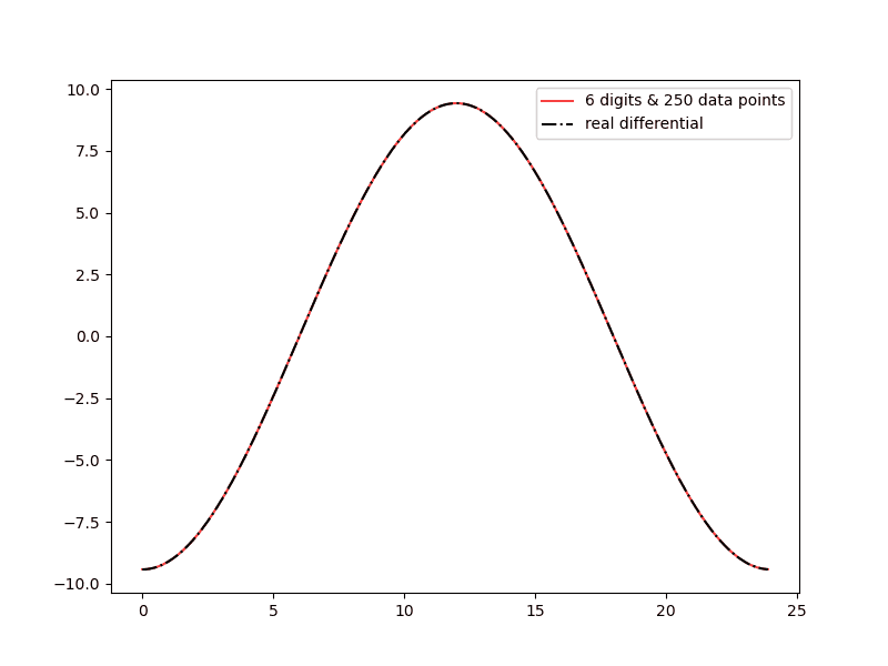
And, even at only 6 digits of precision and 250 data points, our estimated rate of change curve is looking pretty good. Well, at least graphically at a relatively low resolution. Okay that’s it for this bit. Time to move on.

Estimating the Change in Battery Charge

What we are going to do now, is take our charge rate function and use it to get back the state of charge function. In calculus this process is called integration.

We will start by determining the change in charge for some time interval. E.G. 06:00-07:00. And, as we did for the differential, we will be using a second function to determine the change in charge for some very small interval (back to that concept of infinitesimal change).

charge_chg_small()

Let’s start with the latter. Now, the charge rate is defined as follows.

$$ \text{charge rate} \approx \text{average charge rate} = \frac{\text{change in charge}}{\text{time period}} $$

Which in turn gives us the following.

$$ \text{change in charge} \approx \text{charge rate} \times \text{time period} $$

And, our function looks like the following.

... ...
def charge_chg_small(c_fn, r_fn, tm, dt):
  ''' Return the estimate change in battery charge for the
      time period tm to tm+dt
  
    :param c_fn: state of charge function
    :param r_fn: rate of change estimation function
    :param tm: period start time, float 0-24
    :param dt: length of period, float > 0, the smaller the better

    returns: estimate change in state of battery charge
  '''
  # our differential estimating function needs the state of charge function to work
  return r_fn(c_fn, tm) * dt

Let’s look at the result for a dt of 1 hour at 17:00.

... ...
if blk_2b["roc2"]:

  t_st, t_dt = 17, 1
  e_chg = charge_chg_small(soc_fn, est_df, t_st, t_dt)
  print(f"charge_chg_small(soc_fn, est_df, {t_st}, {t_dt}) = {e_chg}")
  a_chg = soc_fn(t_st + t_dt) - soc_fn(t_st)
  print(f"soc_fn({t_st + t_dt}) - soc_fn({t_st}) = {a_chg}")
  print(f"\t% diff est over act: {(100 * (e_chg - a_chg) / a_chg):.2f}%")

And in the terminal I got the following.

(mc-3.14) PS R:\learn\mc\calculus> python txt_loc.py -c roc2
charge_chg_small(soc_fn, est_df, 17, 1) = 2.4393119258165825
soc_fn(18) - soc_fn(17) = 1.2266702535935394
        % diff est over act: 98.86%

Definitely not what we want. Let’s try a difference of 0.01.

(mc-3.14) PS R:\learn\mc\calculus> python txt_loc.py -c roc2
charge_chg_small(soc_fn, est_df, 17, 0.01) = 0.024393119258165827
soc_fn(17.01) - soc_fn(17) = 0.02427392620219848
        % diff est over act: 0.49%

Most certainly an improvement. But we may need to go to a yet smaller dt as we progress.

charge_chg()

Okay, let’s move on to the main charge change function. We split the time period passed in the paramters into smaller periods and use the charge_chg_small() function to calculate the change for each of those smaller intervals. Then we will add them up to estimate the change in charge for the larger interval. Sound familiar?

And, because I am going to need to pass a couple of functions to charge_chg_small those will need to be passed to our current function as well. We will also need to pass start and end times and the desired small interval size. Let’s have a look at a possible solution.

def charge_chg(c_fn, r_fn, st, et, dt):
  ''' Return the estimate change in battery charge for the
      time period st to et
  
    :param c_fn: state of charge function
    :param r_fn: rate of change estimation function
    :param st: period start time, float 0-24
    :param et: period end time, float 0-24
    :param dt: time delta to be used by charge_chg_small, float > 0, the smaller the better
               must divide time period into an even number of smaller periods,
               as we prefer a whole number of intervals

    returns: estimate change in state of battery charge for the specified period
  '''

  t_sm = np.arange(st, et, dt)
  return sum(charge_chg_small(c_fn, r_fn, t, dt) for t in t_sm)

A couple rather simple functions. A wee test, including timing for a range of time deltas.

... ...
  t_st, t_nd, t_dts = 10, 18, [0.1, 0.05, 0.025, 0.01]
  for t_dt in t_dts:
    st = time.perf_counter()
    c_chg = charge_chg(soc_fn, est_df, t_st, t_nd, t_dt)
    nt = time.perf_counter()
    r_chg = soc_fn(t_nd) - soc_fn(t_st)
    print(f"charge_chg(soc_fn, est_df, {t_st}, {t_nd}, {t_dt}) ={ c_chg}")
    print(f"\tsoc_fn({t_nd}) - soc_fn({t_st}) = {r_chg}")
    print(f"\t% diff est over act: {(100 * (c_chg - r_chg) / r_chg):.2f}%")
    print(f"\tcharge_chg() took {(nt - st):.2f} sec")

And in the terminal the test code output was as follows.

(mc-3.14) PS R:\learn\mc\calculus> python txt_loc.py -c roc2
charge_chg(soc_fn, est_df, 10, 18, 0.1) =54.405019377303624
        soc_fn(18) - soc_fn(10) = 54.0
        % diff est over act: 0.75%
        charge_chg() took 0.01 sec
charge_chg(soc_fn, est_df, 10, 18, 0.05) =54.203280165941834
        soc_fn(18) - soc_fn(10) = 54.0
        % diff est over act: 0.38%
        charge_chg() took 0.03 sec
charge_chg(soc_fn, est_df, 10, 18, 0.025) =54.10183224546269
        soc_fn(18) - soc_fn(10) = 54.0
        % diff est over act: 0.19%
        charge_chg() took 0.05 sec
charge_chg(soc_fn, est_df, 10, 18, 0.01) =54.040778434962476
        soc_fn(18) - soc_fn(10) = 54.0
        % diff est over act: 0.08%
        charge_chg() took 0.13 sec

That last combination used 800 time intervals between 10:00 and 18:00. And, the last two combinations were within one decimal point of the real value. Though clearly the last one was by far the best estimate.

Not going to show the results for any other start and end times. But I can assure you, the choice of those times does slightly affect the quality of the estimate. That said, do you, perhaps, see what is going on here.

Visualizing the Process

Initially I am just going to focus on the rate of change curve between 06:00 and 18:00. Hopefully we will see why later.

Now, we are taking some time range and estimating the change in battery charge for that period. We are doing so by multiplying the rate of change at the start time by the total time in the selected interval. Let’s see what that might look like plotted on the rate of change curve for hourly intervals for the above range.

We will assume the rate of change is constant for each hour in the select time period. If we plot the resulting lines as the rate of change curve we will get something like the following.

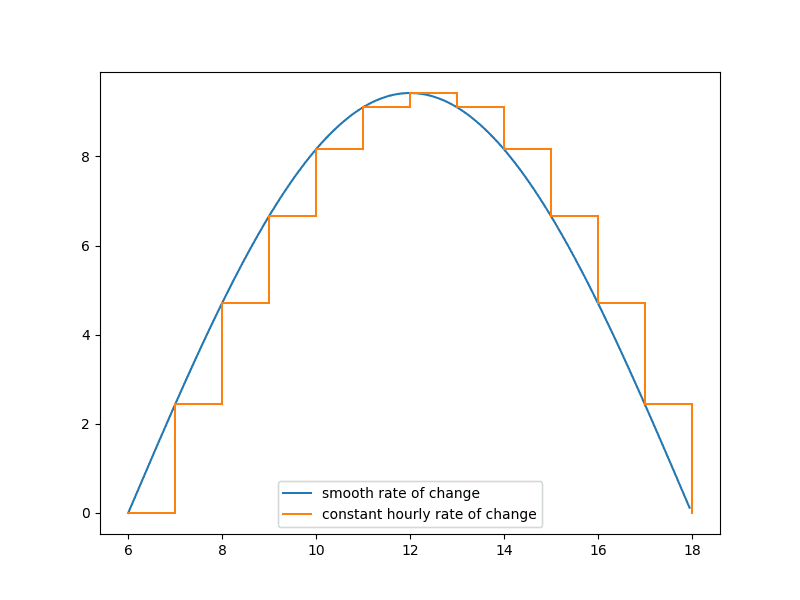
We get a set of steps going up and back down. In step with the rate of charge increasing or decreasing. Each step height is proportional to the steepness of the curve between the start and end points for each time period.

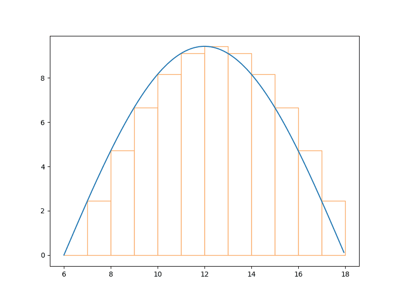
Do you see what is happening? Our calcualation for the total change for each period is the rate of change for that interval times the length of the interval. Now, looking back to grade school geometry, the area of a rectangle is the product of its length and width. Which is exactly what our function is calculating for each interval: the height (the rate of change at the start of the interval) times the time interval. We are calculating the area of an imaginary rectangle. The area of that rectangle represents the change in charge for that time interval. Let’s add that to the visualization.

Now let’s try that with a smaller time interval for each change of charge estimate. Say, 15 minutes.

You can likely see that each rectangle is now going to provide a better estimate of the rate of change for the respective time.

Now let’s use that same interval and plot the curve for the full day. And, you will understand why I initially limited my visualization to the range 06:00 to 18:00.

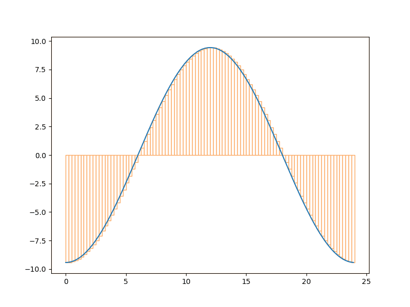
The width of the rectangles in the plot above are in fact the same as those of the plot above it: 15 minutes. The x-axis just has more hours on it, making 15 minutes look smaller. Note: under the curve is somewhat less than self-evident.

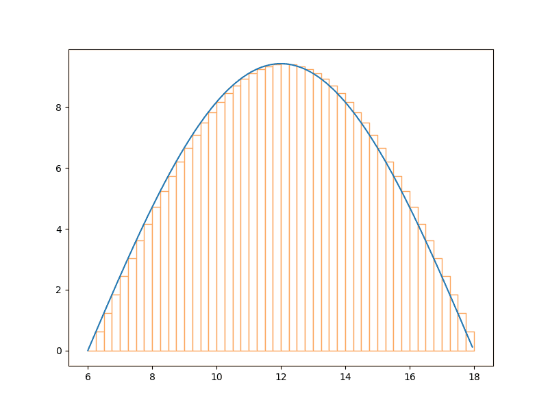
Okay, let’s look at a width of say 36 seconds for each rectangle.

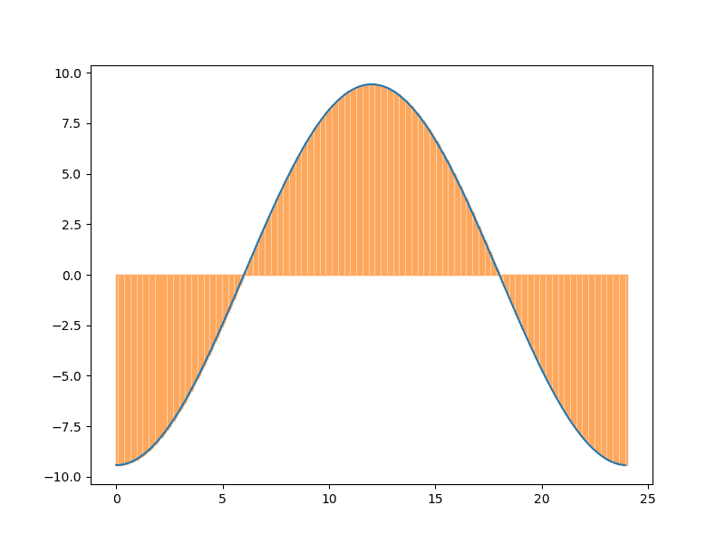
And those imaginary rectangles almost completely cover the space under the curve.

Hopefully you can see that the function charge_chg() will calculate the rate of change for some period of time by summing the areas of all the imaginary rectangles within that time period. That is, it is estimating the area under the curve for that period of time. Which is the change in charge over that period.

Time to see if can now plot the battery charge over time using the charge change function.

Done for Now

But I think I will leave that for another post. I feel comfortable with the content in this one and it did take me some time to produce. Both writing the related code, especially the plots, and the post.

Until next time enjoy your time coding!