Okay, we have a function that gives the estimated change in the battery charge for some period of time. So, we should be able to use that to determine the estimated state of battery charge for any time of the day. Let’s see if we can get that working.
Using Rate of Change Function to Determine Battery Charge
Well, yes our charge change function can tell us how much the battery charge changed between 00:00 and 01:00. But does that tell us what the current battery charge really is?
Let’s just give it a try. Some new boolean control if blocks.
... ...
if blk_2b["roc3"]:

  if i_blk == 0:
    t_st, t_nd, t_dt = 0, 1, 0.01
    # get the change in charge for 00:00 to 01:00 using our change of charge function
    c_chg = charge_chg(soc_fn, est_df, t_st, t_nd, t_dt)
    # get the battery charge at 01:00 from our state of charge function
    b_chg = soc_fn(t_nd)
    print(f"change in charge to 01:00: {c_chg},\nbattery charge at 01:00: {b_chg}")
And, in the terminal the code output the following.
(mc-3.14) PS R:\learn\mc\calculus> python txt_loc.py -c roc3 -i 0
change in charge to 01:00: -9.319085908022023,
battery charge at 01:00: 35.68251437630926
Obviously something is missing. And, of course, that is the state of charge at 00:00. Our change in charge function gives us exactly that. The only way to get the actual battery charge is to add that change to some initial state. We will need to look after that necessity in our future code.
Function Generator
I want the new state of charge function to take a single parameter: the time day for which to determine the current battery state. But the change of charge function that will be used to calculate that value takes a few more parmeters than that. I will be calculating the battery state using the state at 00:00 as the initial state, something the final function will need to know. We will need to pass or hard code the time delta to be used by the change of charge function. I think passing it in is preferable. And that function also requires passing in a couple other functions. (Though I guess we could simply assume the function knows about those other functions and drop a couple of parameters. But…) Only want to do that once, not everytime I call the new state of charge function.
So I have decided to use a technique, from functional programming, called currying.
Currying is a process in functional programming where a function that takes multiple arguments is transformed into a sequence of functions, each taking a single argument. This transformation allows for the gradual application of arguments to a function, enabling partial application and more modular code design.
Introduction to Currying
I know we have already used this technique in previous code/post(s). But until coming across the technique in an article I recently read, I had no idea it had a specific name and a well defined purpose.
I will write a function that returns the desired function having been given all the other values. So, we will have something like mk_soc_fn(c_fn, r_fn, st, dt) which will return a function something like roc_2_soc(tm). Let’s give that go.
I decided to test a few different times in the day and a few different time intervals (for the charge rate estimator) for each. I was curious how the processing time would be affected.
... ...
  def mk_soc_fn(c_fn, r_fn, st, dt):
    i_chrg = c_fn(st)
    def roc_2_soc(tm):
      c_chg = charge_chg(c_fn, r_fn, st, tm, dt)
      return(i_chrg + c_chg)
    return roc_2_soc
... ...
  if i_blk == 1:
    # let's test a few times and a few values for the rate of change time interval
    # checking times for each interval
    tms = [4, 10, 14, 20]
    tis = [.01, .005, .0025, .001]
    params = itertools.product(tms, tis)
    p_dts = tis[1:]
    for dt in tis:
      roc_2_soc = mk_soc_fn(soc_fn, est_df, 0, dt)
      print(f"using time interval (dt) of {dt}")
      for tm in tms:
        if dt in p_dts:
          t_st = time.perf_counter()
        e_soc = roc_2_soc(tm)
        if dt in p_dts:
          t_nd = time.perf_counter()
        r_soc = soc_fn(tm)
        e_err = 100 * (e_soc - r_soc) / r_soc
        print(f"\troc_2_soc({tm}) = {e_soc} ?= soc_fn({tm}) = {r_soc} ({e_err:.2f}%)")
        if dt in p_dts:
          print(f"\t\troc_2_soc took ~ {(t_nd - t_st):.3f} to run")
And, in the terminal I got the following.
(mc-3.14) PS R:\learn\mc\calculus> python txt_loc.py -c roc3 -i 1
using time interval (dt) of 0.01
        roc_2_soc(4) = 13.799541996026061 ?= soc_fn(4) = 13.823085463760208 (-0.17%)
        roc_2_soc(10) = 26.912076102389026 ?= soc_fn(10) = 27.000000000000004 (-0.33%)
        roc_2_soc(14) = 62.912055148528935 ?= soc_fn(14) = 62.99999999999999 (-0.14%)
        roc_2_soc(20) = 76.15333411314384 ?= soc_fn(20) = 76.17691453623979 (-0.03%)
using time interval (dt) of 0.025
        roc_2_soc(4) = 13.764292563752004 ?= soc_fn(4) = 13.823085463760208 (-0.43%)
                roc_2_soc took ~ 0.026 to run
        roc_2_soc(10) = 26.780228515020205 ?= soc_fn(10) = 27.000000000000004 (-0.81%)
                roc_2_soc took ~ 0.061 to run
        roc_2_soc(14) = 62.78009961227369 ?= soc_fn(14) = 62.99999999999999 (-0.35%)
                roc_2_soc took ~ 0.089 to run
        roc_2_soc(20) = 76.11789770917186 ?= soc_fn(20) = 76.17691453623979 (-0.08%)
                roc_2_soc took ~ 0.117 to run
using time interval (dt) of 0.0025
        roc_2_soc(4) = 13.817196761398595 ?= soc_fn(4) = 13.823085463760208 (-0.04%)
                roc_2_soc took ~ 0.249 to run
        roc_2_soc(10) = 26.97801724500829 ?= soc_fn(10) = 27.000000000000004 (-0.08%)
                roc_2_soc took ~ 0.609 to run
        roc_2_soc(14) = 62.97801556772102 ?= soc_fn(14) = 62.99999999999999 (-0.03%)
                roc_2_soc took ~ 0.866 to run
        roc_2_soc(20) = 76.17102226589384 ?= soc_fn(20) = 76.17691453623979 (-0.01%)
                roc_2_soc took ~ 1.223 to run
using time interval (dt) of 0.001
        roc_2_soc(4) = 13.820730118659313 ?= soc_fn(4) = 13.823085463760208 (-0.02%)
                roc_2_soc took ~ 0.633 to run
        roc_2_soc(10) = 26.991206861445473 ?= soc_fn(10) = 27.000000000000004 (-0.03%)
                roc_2_soc took ~ 1.524 to run
        roc_2_soc(14) = 62.99120626364586 ?= soc_fn(14) = 62.99999999999999 (-0.01%)
                roc_2_soc took ~ 2.187 to run
        roc_2_soc(20) = 76.17455749225712 ?= soc_fn(20) = 76.17691453623979 (-0.00%)
                roc_2_soc took ~ 3.027 to run
I didn’t expect the processing time to increase so significantly as the time got later in the day. Though I did expect the processing time to increase as the time interval decreased in size.
Going to estimate how long processing a full day might take. I will use the average processing time for 04:00 and 20:00. Hopefully a decent estimate for each time of day. Then I will assume a range of 100 times will be calculated to plot the graph we are after.
PS R:\learn\mc> perl -e "print (((0.117 - 0.026) / 2) * 100);"
4.55 @ interval of 0.025
PS R:\learn\mc> perl -e "print (((1.123 - 0.249) / 2) * 100);"
43.7 @ interval of 0.0025
PS R:\learn\mc> perl -e "print (((3.027 - 0.633) / 2) * 100);"
119.7 @ interval of 0.001
Generating Full Day
I am sure the processing time will in fact be longer than the numbers above. But, certainly a big jump for those much smaller estimator time intervals.
Okay, let’s generate the data for a full day, using perhaps a couple different time intervals. Will also plot estimated state of charge curve over a plot of the actual state of charge curve. Will plot the latter in a lighter colour with a much thicker line width (my aging eyes need the help).
... ...
  if i_blk >= 2:
    t_dt, il = .025, "a"
    if i_blk == 3:
      t_dt, il = .01, "b"
    elif i_blk == 4:
      t_dt, il = .005, "c"
    roc_2_soc = mk_soc_fn(soc_fn, est_df, 0, t_dt)
    tms = np.arange(0, 24.25, .25)
    print(len(tms), "times")
    t_st = time.perf_counter()
    socs = [roc_2_soc(tm) for tm in tms]
    t_nd = time.perf_counter()
    print(f"{len(socs)} socs\n\ttook {(t_nd - t_st):.2f} secs to create soc data at dt of {t_dt}")

    socs2 = soc_fn(tms)

    fig, ax = plt.subplots(figsize=(8, 6))
    ax.plot(tms, socs2, label="actual state of charge", lw=8, alpha=.4)
    ax.plot(tms, socs, label=f"est state of charge ({t_dt})", c="k")
    ax.legend()
    lx, ly = (0, 24), (0, 100)
    ax.set(xlim = lx, ylim = ly, autoscale_on = False)

    if blk_2b["sv_plt"]:
      fig.savefig(f"img/roc3_{i_blk + 1}{il}.png")
    plt.show()
Time Interval of 0.025
(mc-3.14) PS R:\learn\mc\calculus> python txt_loc.py -c roc3 -i 2
97 times
97 socs
        took 7.12 secs to create soc data at dt of 0.025
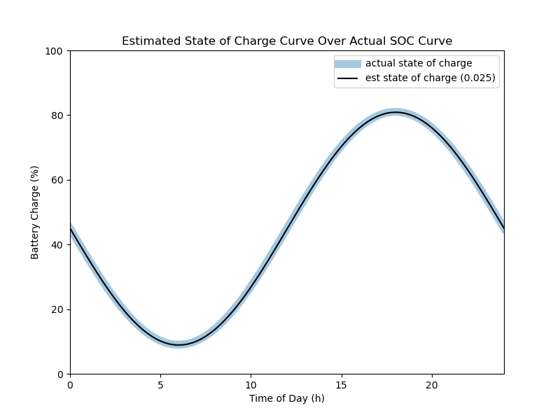
Not a bad fit at this resolution. Can just see a little bit of discrepancy between roughly 07:00 and 17:00. Estimate is pretty well centered other times of the day.
Time Interval of 0.01
(mc-3.14) PS R:\learn\mc\calculus> python txt_loc.py -c roc3 -i 3
97 times
97 socs
        took 17.71 secs to create soc data at dt of 0.01
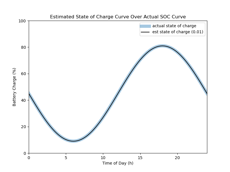
Estimate much more centered (at this resolution).
Time Interval of 0.005
(mc-3.14) PS R:\learn\mc\calculus> python txt_loc.py -c roc3 -i 4
97 times
97 socs
         took 34.46 secs to create soc data at dt of 0.005
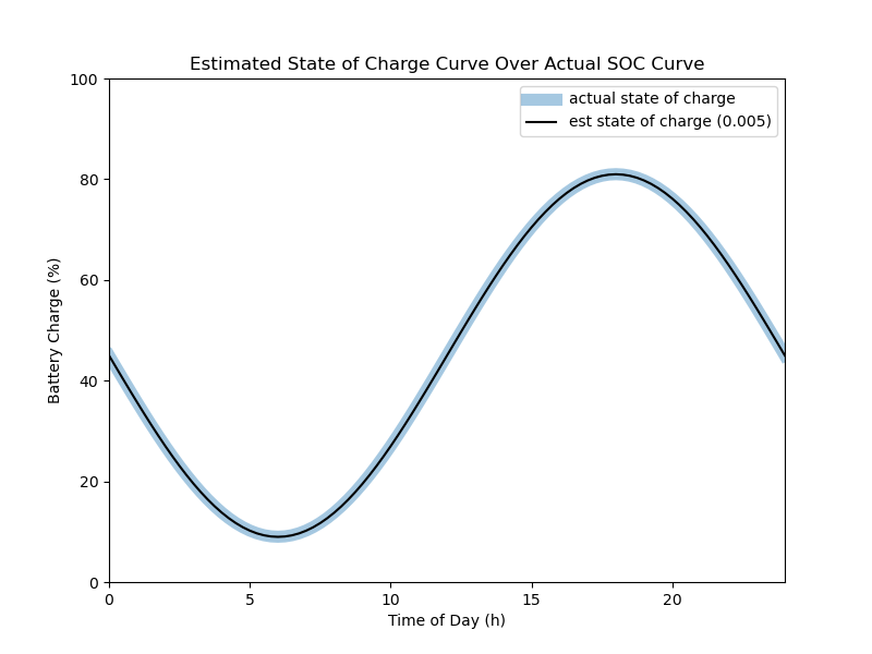
Hard to tell the difference between those last two. But I do believe there is a slight improvement in the middle of the day for the last one.
A Possible Improvement
You may recall that in our prior work, the function to estimate the differential took a parameter specifying the degree of precision (number of decimals) to which we wanted the value calculated. We could likely do the same here, but I expect the time to completion would be rather lengthy for any meaningful number of digits of precision. And, personally don’t see any reason to experiment any further.
I Believe We Are Done
In calculus one of the key objectives of the integral is to recover the original function. In our case, we would, mathematically, integrate the charge rate of change function (the differential of the state of charge function) to get back the state of charge function. Since we are avoiding that kind of mathematics I won’t bother doing so (assuming I could).
This has been a fun little project. It forced me to learn a bit more about coding and plotting. And, reminded me of my much younger days in college. All in all, not bad for a relatively easy going project.