After that side-trip looking at a bit of calculus, I wasn’t sure what I would do next. Still not quite ready to go back and tackle coding a transformer model. But, I have for some time been thinking about generating music programmatically. I know it won’t produce anything like the classical masterpieces I typically listen to while coding or working on this blog. But, it strikes me as a project I might be interested in enough to pursue for at least a few weeks. So here we go.

I am going to start slow and easy. I.E. I will start by looking at what exactly a musical note is in terms of mathematics and/or numbers. Then probably what a chord is and what other notes might go well with a chord. Then, down the road, we will likely need to consider some musical concepts. Then…

uv

But first, a new Python package and project manager: uv.

I have been reading about this package manager for a while now. And, a lot of the people writing those articles have moved from conda to uv. So, I figured it was time I had a look. And, as I was starting a new project, figured now was as good a time as any.

Installation

Not sure why but I didn’t want uv installing itself in the default location.

By default, uv is installed in the user executable directory.
The uv installer

In my case that would be: %USERPROFILE%\.local\bin. I am going to put it elsewhere. And I will be using Powershell as winget can’t alter the installation location. That command looks like the following. Note that is one continuous line, no line break.

powershell -ExecutionPolicy ByPass -c {$env:UV_INSTALL_DIR = "C:\Custom\Path";irm https://astral.sh/uv/install.ps1 | iex}

My location doesn’t really matter, and yours would, I am sure, be different.

PS R:\learn> powershell -ExecutionPolicy ByPass -c {$env:UV_INSTALL_DIR = "xxxx";irm https://astral.sh/uv/install.ps1 | iex}
downloading uv 0.10.9 (x86_64-pc-windows-msvc)
installing to xxxx
  uv.exe
  uvx.exe
  uvw.exe
everything's installed!

And, after restarting my terminal session(s):

PS R:\learn> uv --version
uv 0.10.9 (f675560f3 2026-03-06)

So, looks to be installed. Let’s find out.

New Project Environment

Let’s create that new project virtual environment. I want the environment to use Python 3.14 or better. So need to specify that or uv will default to whatever my default version is (3.6.x I believe).

PS R:\learn> uv init e_music --python 3.14
Initialized project `e-music` at `R:\learn\e_music`
PS R:\learn> Get-ChildItem -Path e_music

    Directory: R:\learn\e_music

Mode                 LastWriteTime         Length Name
----                 -------------         ------ ----
-a----        2026-03-12     12:43            109 .gitignore
-a----        2026-03-12     12:43              5 .python-version
-a----        2026-03-12     12:43             85 main.py
-a----        2026-03-12     12:43            153 pyproject.toml
-a----        2026-03-12     12:43              0 README.md

And in pyproject.toml we have the following.

[project]
name = "e-music"
version = "0.1.0"
description = "Add your description here"
readme = "README.md"
requires-python = ">=3.14"
dependencies = []

And a very basic main.py for us to use/test the project initailization.

def main():
    print("Hello from e-music!")


if __name__ == "__main__":
    main()

The init command, in fact, did not yet create a virtual environment. That will happen the first time we run our main project python module.

PS R:\learn> Set-Location -Path e_music
PS R:\learn\e_music> uv run main.py
Using CPython 3.14.3
Creating virtual environment at: .venv
Hello from e-music!
PS R:\learn\e_music> Get-ChildItem

    Directory: R:\learn\e_music

Mode                 LastWriteTime         Length Name
----                 -------------         ------ ----
d-----        2026-03-12     12:51                .venv
-a----        2026-03-12     12:43            109 .gitignore
-a----        2026-03-12     12:43              5 .python-version
-a----        2026-03-12     12:43             85 main.py
-a----        2026-03-12     12:43            153 pyproject.toml
-a----        2026-03-12     12:43              0 README.md
-a----        2026-03-12     12:51            127 uv.lock

When I ran main.py, uv created the virtual environment and installed Python version 3.14.3.

Also, git is initialiaed for us. You did see the .gitignore file in the first directory listing.

PS R:\learn\e_music> git st
On branch master

No commits yet

Untracked files:
  (use "git add <file>..." to include in what will be committed)
        .gitignore
        .python-version
        README.md
        main.py
        pyproject.toml
        uv.lock

nothing added to commit but untracked files present (use "git add" to track)

I will look at initializing a new github repo and commit the above files. Though not sure why uv.lock should be committed. But uv did not include it in .gitignore so I am guessing there is a reason. Well, here’s what uv has to say.

uv.lock is a cross-platform lockfile that contains exact information about your project’s dependencies. Unlike the pyproject.toml which is used to specify the broad requirements of your project, the lockfile contains the exact resolved versions that are installed in the project environment. This file should be checked into version control, allowing for consistent and reproducible installations across machines.
Working on projects

Time to move onto making sounds (hopefully pleasant ones). Though lot’s of introductory discussion before we try making some music.

Sound

I expect we all pretty much know what sound is. A vibration in the air which when it arrives at our ears as a wave causes the ear drums to vibrate. Those vibrations are interpreted by our physiology as sound. Pleasant or otherwise. If there’s no one to hear it does a falling tree make a sound?

For our purposes I am going to say yes. Because sound, heard or otherwise, is just a vibration in some medium. Be that air, water or jello. So, let’s start by looking at what that vibration might be.

Repeating Waves

Now these waves have some properties of interest to us. The one we likely know best is frequency. That is, the number of complete waves to pass some point in a period of time (for our case usually a second). Different sounds (e.g. musical notes) have different frequencies. And humans perceive sounds with higher frequencies to be higher pitched (e.g. left hand keys on a piano versus the right hand keys or a tenor versus a soprano).

But there is also amplitude. Amplitude, the height of the wave, determines the strength of the vibration. In our case, the amplitude correlates to our perception of loudness. Then there is wavelength: how far a vibration’s compression travels before the next compression. In our case, that would be the distance between adjacent crests. Similarly there are period, speed and phase, but I don’t at this point think those properties will be relevant to our project. Though I should add, we will likely only be interested in periodic waves.

Music Notes

In my world of music, there are twelve notes in every octave.

An equal temperament is a musical temperament or tuning system that approximates just intervals by dividing an octave (or other interval) into steps such that the ratio of the frequencies of any adjacent pair of notes is the same. This system yields pitch steps perceived as equal in size, due to the logarithmic changes in pitch frequency.

In classical music and Western music in general, the most common tuning system since the 18th century has been 12 equal temperament (also known as 12-tone equal temperament, 12 TET or 12 ET, informally abbreviated as 12 equal), which divides the octave into 12 parts, all of which are equal on a logarithmic scale, with a ratio equal to the 12th root of 2, ${\textstyle {\sqrt[{12}]{2}}} ≈ 1.05946$. That resulting smallest interval, ⁠1/12⁠ the width of an octave, is called a semitone or half step. In Western countries the term equal temperament, without qualification, generally means 12 TET.

In modern times, 12 TET is usually tuned relative to a standard pitch of 440 Hz, called A 440, meaning one note, A, is tuned to 440 hertz and all other notes are defined as some multiple of semitones away from it, either higher or lower in frequency.

Equal temperament

And those twelve notes in each octave would be: C, C#, D, D#, E, F, F#, G, G#, A, A#, and B. Starting with C is a musical convention based on the piano. I will be using the octave, 4, starting at middle C as my base set of notes. Though based on the above quote, the A4 frequency, 440Hz, will be the base value from which the frequency of all other notes will be calculated.

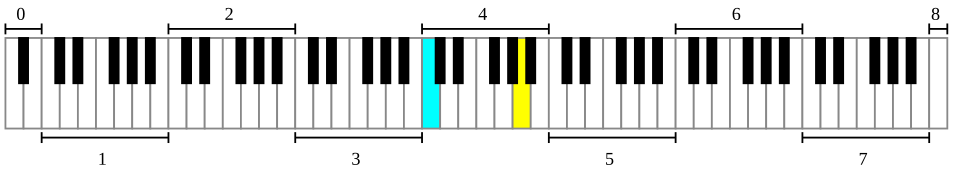
image of 88 key piano with the octaves numbered and middle C highlighted — Image from Octave

Let’s start by looking at the wave that might generate the note middle C or C4. I will go with the fact that Middle C (aka C4) is 9 semi-tones below A4.

$$\text{note frequency} = 440 * 2^{\frac{n}{12}}$$ $$\text{where: n is the number of semitones from A4}\\\\\text{- negative if note is to the left on a piano, postive otherwise}$$

Get Frequency Function

Figured I should write a function to get a note’s frequency so I understand how the 12 TET works. Might be a throw away experiment.

But, I also want to be able to specify the equivalent octave on the piano. So, I am going to identify a note by the symbol (e.g. C or F#) and an octave number appended to it. So, middle C will be C4, A above it A4. The F# below middle C will be F#3. If no octave number is appended it will default to 4. For now I will assume the octave number will always be a single digit from 0 to 8. Though only one note in 8th octave on a piano. But, not currently enforcing that in the function.

def get_note_freq(sym: str) -> int:
  # n_syms = ("C" ,"C#","D" ,"D#","E" ,"F" ,"F#","G" ,"G#", "A", "A#", "B")
  n_pos = {'C': -9, 'C#': -8, 'D': -7, 'D#': -6, 'E': -5, 'F': -4, 'F#': -3, 'G': -2, 'G#': -1, 'A': 0, 'A#': 1, 'B': 2}
  ref_frq = 440
  ref_oct = 4
  n_ptch = 1
  if sym[-1].isdigit():
    n_oct = int(sym[-1]) - ref_oct
    if n_oct < 0:
      n_ptch = 0.5**abs(n_oct)
    elif n_oct > 0:
      n_ptch = 2**n_oct
    n_sym = sym[:-1]
  return ((ref_frq * 2**(n_pos[n_sym]/12)) * n_ptch)


def main():
  for t_nt in ["A", "A4", "A3", "C", "C5", "C6", "G#4", "G#3"]:
    print(f"get_note_freq({t_nt}): {get_note_freq(t_nt)}")

And, in the terminal I got the following.

PS R:\learn\e_music> uv run main.py
get_note_freq(A): 440.0
get_note_freq(A4): 440.0
get_note_freq(A3): 220.0
get_note_freq(C): 261.6255653005986
get_note_freq(C5): 523.2511306011972
get_note_freq(C6): 1046.5022612023945
get_note_freq(G#4): 415.3046975799451
get_note_freq(G#3): 207.65234878997256

Which as far as I can tell is correct.

Wave Function

Okay, we have the frequency, but what’s that wave function going to look like. Well, for now it’s going to look like a sine wave. But, we will need to adjust the standard sine wave to account for the frequency of our note and likely the desired amplitude. And one more, important, consideration: sampling frequency (nothing to do with the note’s frequency).

First let’s consider the data we want to use to generate the sound’s wave function. We will be using the sine function (likely numpy) which takes an angle, in radians, to generate a value of the sine. The sine has a period of $2\pi$. We want to specify a frequency then get the value of the sine function for that frequency at some number of points in the length of time the note is to be played.

Now, if we use a time, $t$, as a decimal in the range $0 - 1$ seconds, then $np.sin(2\pi * t)$ for every $t$ in that range would give us one complete cycle of the sine function. If we multiply the sine’s input by our frequency, $2\pi * t * f$, we will get $f$ cycles in the same time period compared to the single cycle for $2\pi * t$.

Let’s have a quick look at a simple test case.

import numpy as np
import matplotlib.pyplot as plt
... ...
def main():
  do_t1 = False
  do_t2 = True
... ...
  if do_t2:
    # visualize modifying frequency for sine curve
    fig, (ax1, ax2) = plt.subplots(2, figsize=(8, 6), sharex=True)

    # plot base curve for a series of times
    ts = np.arange(0, 1, 0.01)
    st1 = np.sin(2 * np.pi * ts)
    s_base = ax1.plot(ts, st1)
    ax1.set(ylabel="Sine",
        title="One Cycle of the Sine Curve (Frequency 1 Hz)")

    # plot sine curve with a higher frequency
    frq = 5
    p_f_pth = f"img\\sine_frq_{frq}.png"
    st2 = np.sin(2 * np.pi * frq * ts)
    s_frq = ax2.plot(ts, st2)
    ax2.set(xlabel="Time", ylabel="Sine",
        title=f"Sine Wave with Frequency of {frq} Hz")

    fig.tight_layout()
    fig.savefig(p_f_pth)

  plt.show()

And the resulting plot.

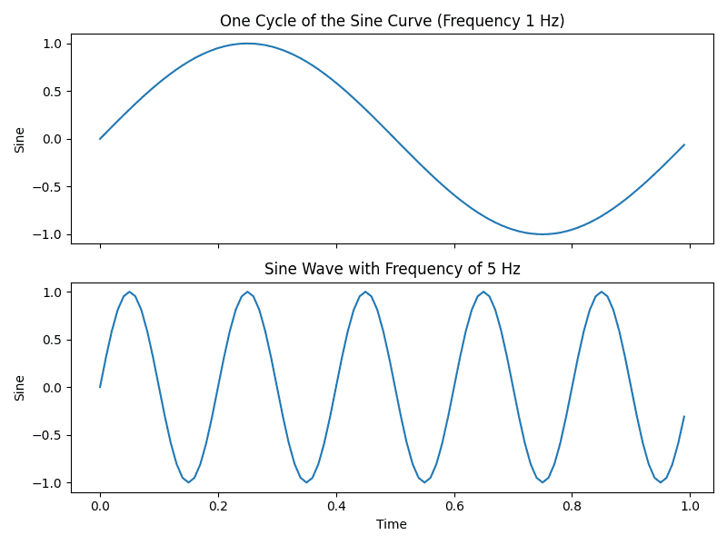
image comparing sine curves with a frequency of 1 and 5

And, that seems to work as expected.

Sampling Rate

Before moving on to playing a note (or eventually music), we need to sort one more thing: sampling rate.

In all of our plotting of sine functions the last several posts (in the calculus series and earlier), we have always selected a set of values from all those possible on the x-axis. We then calculate the sine values for those points. Those two sets of data are passed to matplotlib for it to generate the plot (a nice smooth curve in our plots to date). We are doing that because there is just no way we could calculate the sine value for every point on the x-axis. Given there would be an infinite number of decimal/float values between 0 and 1. We’d run out of memory and time.

So, we use a sample of of the available points. We will need to do the same for the sine curves used to generate notes in our electronically generated music. Now for the state of charge curve (a modified sine curve) in the calculus series I used 240 data points. And, in the plot above, 100 data points. The latter is a sampling rate of 100 for 1 second of time or 100Hz.

In our case, i.e. sound, we need to be aware of what the sampling rate does or does not.

The number of samples captured per second determines the frequency range that can be captured and reproduced. Owing to something called the ‘Nyquist theorem‘, the highest frequency that can be represented by digital audio is half the value of the sample rate.

What is the best audio sample rate? 44.1, 48, 96? Sample rate explained

Humans, well the ones with the best possible hearing, can hear frequencies in the range 20Hz to 20kHz. So, most electronic music uses a sampling rate of 44.1kHz. Which equates to a maximum frequency of ~22kHz. Good enough for our purposes, so that’s what we will go with.

Now I know the range of frequencies on an 88-key piano are in the range 27.5Hz to 4.186kHz. A piccolo can hit a high of 5kHz. So why the big sampling rate? Not going to get into it, but I believe the answer is harmonics. Pretty much every instrument produces additional sound waves with frequencies at interger multiples of the base note frequency. The amplitude of the harmonic waves decreases with frequency. We perceive harmonics as part of a single sound, improving its richness and complexity.

This One Done

I was going to write code to play that C4 note. But I have not yet sorted which approach or library to use to get python to produce sound. Will do some investigating and/or playing around between now and starting the next post.

Until then, may you get around to producing music faster than I appear to be doing so.

Resources

uv Introduction
What is the best audio sample rate? 44.1, 48, 96? Sample rate explained
Understanding Harmonics: The Science Behind Rich And Complex Sounds

Too Old To Code

eMusic

uv